Scalability design

Lens stores two kinds of data. Traces and request logs live in ClickHouse, which is append-only and grows with traffic. Lenses, investigation jobs, findings, and worker state live in PostgreSQL, which is small and changes often. Each design rule below keeps the cost of a common operation tied to the work it actually does, so it does not grow with total retention, total traffic, or the number of lenses

Operation	Store	Cost grows with	Does not grow with
Sample a window	ClickHouse	Spans in the window plus 7 days of slack	Retention, number of pages
Read one trace	ClickHouse	Partitions from the trace start minus 7 days to now	Retention for recent traces, other teams
Claim a job	PostgreSQL	Due lenses, read 20 at a time	Total lenses, lenses not due
Heartbeat a job	PostgreSQL	Size of the lens document today; a narrow lease row in the target design	Number of lenses

The charts and tables on this page come from a local benchmark that runs the Lens SQL from before and after each change against real ClickHouse and PostgreSQL. Every timing is repeated and reported as a median with its p10 to p90 spread, and Benchmark methodology lists the hardware, versions, dataset and run counts. They show how cost grows with data size on one machine and are not production latency targets

Every trace query is bounded by time

otel_traces is partitioned by day and ordered by (TeamId, ServiceName, Timestamp, TraceId). ClickHouse skips data only when a query constrains those columns, so a query that filters on a derived expression such as EngineReceivedMs, or that has no time filter at all, has to open every partition the team has retained. Its cost then grows with retention even when the answer covers a single day

Every Lens query against otel_traces and spend_logs must therefore put a direct range on Timestamp or start_time on top of its own logic. Spans can start before the window being sampled, and they can arrive late, so the lower bound carries a fixed slack of 7 days. That covers multi-day coding agent sessions while still skipping the rest of retention. The upper bound applies only where it cannot hide spans that later checks depend on. For example, the sample query still sees later spans so that traces still in progress stay excluded

A 24 hour sample with the time bound reads about 1.0M rows at every retention from 7 to 90 days. Without it, the same single query reads 3.2M rows at 30 days and 9.4M at 90 days

Samples are selected once per job

A sample is a deterministic selection over every trace eligible in the window. It needs the eligible count and the selection order, and both require the full eligible set. Paging that query 100 rows at a time recomputes the full set on every page, so a single sample costs pages times window size

The worker requests the selection in pages of 10,000, so a normal sample takes one query, then freezes it on the job. Later reads use the frozen selection and do not query ClickHouse again. If a page would exceed the response limit, the worker retries the same cursor with a smaller page. Previews in the dashboard still page, but each page is time bounded

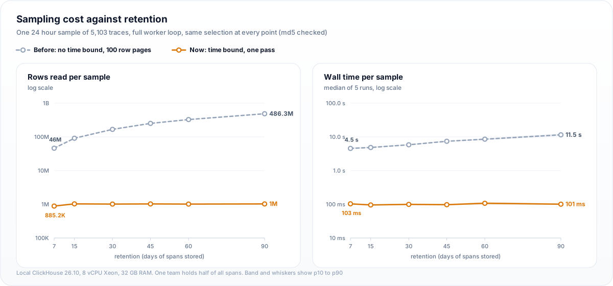
The chart runs the full worker sample loop for the same 24 hour window, about 5,100 traces selected, at six retention sizes. Before, rows read grow from 46M at 7 days to 486M at 90 days and the loop takes 4.5 s to 11.5 s. Now every retention reads about 1.0M rows in about 100 ms. Every timed run of both versions selected the same traces in the same order

The table separates the two changes at 30 and 90 days, median of 5 runs:

Retention	Query	Page size	Queries	Rows read	Bytes read	Median time
30 days	before	100	52	167.2M	8.4 GB	5.2 s
30 days	before	10,000	1	3.2M	162 MB	130 ms
30 days	time bounded	100	52	52.8M	3.4 GB	4.2 s
30 days	time bounded	10,000	1	1.0M	66 MB	97 ms
90 days	before	100	52	486.3M	22.2 GB	9.4 s
90 days	before	10,000	1	9.4M	427 MB	199 ms
90 days	time bounded	100	52	53.2M	3.4 GB	4.2 s
90 days	time bounded	10,000	1	1.0M	66 MB	105 ms

Most of the gain comes from selecting once, and the time bound is what keeps the cost flat as retention grows. Together they cut a 90 day sample from 486M rows to 1.0M

Single trace reads are keyed and windowed

Reading one trace is a point lookup. A bloom filter on TraceId narrows the read to the granules that hold the trace, and pages return at most 40 spans, ordered and cursored by SpanId, with span content truncated to a fixed budget. Each read therefore returns a bounded payload however large the trace is

The bloom filter is still checked on every granule of the team. Lens reads pass the trace start time saved with the sampled execution, minus the same 7 day slack, so the lookup opens only the partitions that can hold the trace

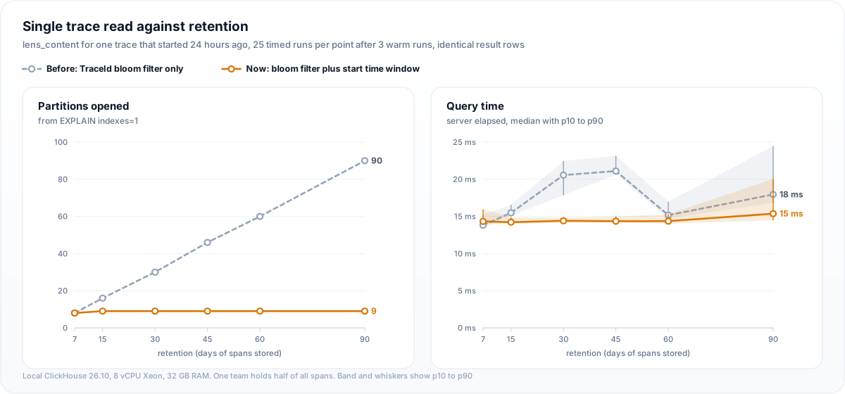
For a trace that started a day ago, the unbounded read opens every partition the team has, 8 at 7 days of retention and 90 at 90 days. The bounded read opens at most 9 at every retention. On this machine opening a partition is cheap, so the latency gain is small: the bounded read stays near 14 ms while the unbounded one moves between 14 and 21 ms. Both return identical spans

Content read for one trace by trace age, median of 25 warm runs:

Retention	Trace age	Partitions before / now	Rows read before / now	Median before / now
30 days	1 day	30 / 9	20,055 / 7,101	13.4 ms / 14.4 ms
30 days	15 days	30 / 23	13,378 / 6,693	12.8 ms / 17.1 ms
90 days	1 day	90 / 9	26,633 / 6,654	16.9 ms / 14.4 ms
90 days	15 days	90 / 23	13,369 / 6,694	16.5 ms / 17.5 ms
90 days	45 days	90 / 53	28,134 / 21,462	16.1 ms / 23.1 ms
90 days	85 days	90 / 90	13,352 / 13,352	16.5 ms / 17.8 ms

The bound keeps the partitions a read opens tied to the trace's age, and that is what lets recent reads stay flat as retention grows. Lens mostly reads traces it has just sampled, so the common case is the recent one. Older traces open more partitions, and at 15 and 45 days the bounded read was 1 to 7 ms slower in this run even though it read fewer rows. A trace near the end of retention opens the same partitions as before

Scheduling does not scan every lens

A worker claim must find one due job, and that cost should not grow with the number of lenses. Before this design a claim loaded and validated every lens, which took 1.1 s with 200 lenses and 5.4 s with 800, per attempt. Each lens now keeps the next time it needs a worker in a due_at column with an index. That is when its queued job was created, when its running job's lease expires, or its next scheduled run. Every full update of a lens writes due_at in the same statement, so the column cannot drift from the document

A claim reads pages of up to 20 due lenses in (due_at, id) order until it claims one or exhausts the queue. A worker that loses the race for one moves on to the next instead of retrying against a lens another worker just took. Lenses created before the column existed start with a due_at in the past, and the first claim that looks at one writes its real value

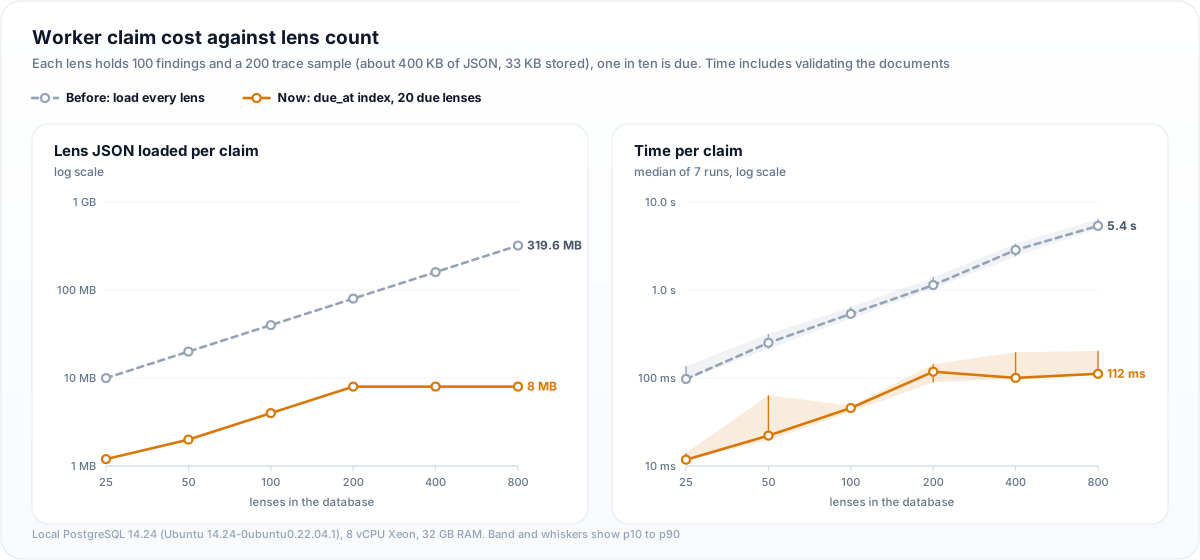
In the chart each lens holds 100 findings and a 200 trace sample, about 400 KB of JSON, and one lens in ten is due. A full scan loads every document, so its cost doubles each time the lens count doubles. The due query loads at most one page of 20 candidates, so after 200 lenses it stays at 8 MB and about 110 ms however many lenses exist. Time includes validating the documents, median of 7 runs:

Lenses stored	Due	Loaded with the due queue	Claim time	Loaded by a full scan	Claim time
25	3	1.2 MB (3 lenses)	12 ms	10 MB (25 lenses)	97 ms
100	10	4.0 MB (10 lenses)	46 ms	40 MB (100 lenses)	535 ms
200	20	8.0 MB (20 lenses)	118 ms	80 MB (200 lenses)	1.1 s
400	40	8.0 MB (20 lenses)	100 ms	160 MB (400 lenses)	2.8 s
800	80	8.0 MB (20 lenses)	112 ms	320 MB (800 lenses)	5.4 s

Hot state is narrow and history is append-only

A heartbeat or progress update should touch only what changed. Today a lens and all of its jobs, findings, and reservations are stored as one JSONB document. Every heartbeat rewrites the whole document, and every update to a lens contends on the same row

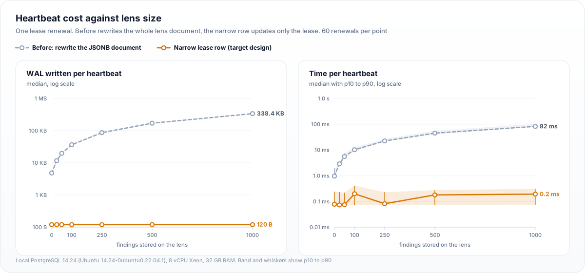
One lease renewal, median of 60 renewals per size:

Findings	Sampled traces	Stored document	Document rewrite	Lease row update
0	50	4.0 KB	0.96 ms, 4.8 KB WAL	0.08 ms, 120 B WAL
100	200	33 KB	10.2 ms, 36 KB WAL	0.20 ms, 120 B WAL
250	500	79 KB	22.4 ms, 87 KB WAL	0.08 ms, 120 B WAL
500	1,000	155 KB	45.1 ms, 171 KB WAL	0.18 ms, 120 B WAL
1,000	2,000	308 KB	82.1 ms, 338 KB WAL	0.19 ms, 120 B WAL

The rewrite costs grow in step with the document, because PostgreSQL writes a new copy of the whole JSONB value on every update. The lease row stays at one small tuple however much history the lens has

The target design moves leases and job progress into narrow rows. Findings, occurrences, and evidence become rows that are only ever appended, and run and review history gets a retention cutoff

Trace lists use a time-ordered rollup

The trace list aggregates spans into one row per trace. Ordering that rollup by (TeamId, ApiKeyHash, TraceId) with no time column forces every page to aggregate the team's whole retention before filtering by start time. In the benchmark a one hour trace list page read all 150K of the team's traces in the rollup. The target design orders the rollup by team and trace start, so a page reads only the window it shows. This requires a new table and a backfill, so it ships separately from the query changes above

Benchmark methodology

All measurements ran on one machine with 8 vCPUs (Intel Xeon Platinum 8559C) and 32 GB of RAM, using ClickHouse 26.10.1 as a single local server and PostgreSQL 14.24, with nothing else under load. The ClickHouse tables come from the Lens migrations, and each query is the exact SQL file from the code before and after the change, bound with the same parameters the proxy sends

The ClickHouse dataset is 18M synthetic spans over 90 daily partitions, about 200K spans a day, spread over 6 teams with one owning half of them. Every trace has 20 spans with attribute maps and message content. The smaller retentions of 7, 15, 30, 45 and 60 days are copies of the newest days of the same data, so every retention holds identical spans for the window being sampled. The sample window is the 24 hours that end at the newest span. read_rows and read_bytes come from system.query_log, partitions opened come from EXPLAIN indexes = 1, and times are wall clock at the client. Each sample loop ran once to warm the cache and then 5 times, and each trace read ran 3 times to warm up and then 25 times. The sample result is hashed on every run to check that both versions select the same traces in the same order

The PostgreSQL table matches LiteLLM_Lens with its due_at index. Lens documents are built with the Lens Pydantic models, and each finding has 5 evidence quotes and 50 occurrences. Claim time covers the query plus validating every returned document, median of 7 runs after a warm-up. Heartbeat WAL is the difference in pg_current_wal_lsn() around each update, after a checkpoint, over 60 renewals spread across 20 lenses. The lease row is the narrow table the target design uses: an id, a lease timestamp and a version

These results describe how cost scales on one machine with warm caches. Production clusters have more cores and slower or remote disks, so absolute times will differ, while rows read, partitions opened, bytes loaded and WAL written depend on the data and should carry over

Load tests

Each design rule above has a load test that fails if the rule is broken. Each test measures the cost of an operation, adds data the operation should never touch, and asserts that the cost does not grow. Each was also run with its optimization reverted to confirm that it fails

Test	Adds	Measured with the design	With the design reverted
lens_sample_reads_scale_with_window_not_retention	24 older days of spans	30,000 rows read before and after	fails, 30,000 grows to 110,000
lens_content_reads_scale_with_trace_not_retention	24 older days under the same trace id	2,000 rows read before and after	fails, 2,000 grows to 50,000
test_lens_claim_reads_scale_with_due_lenses_not_total_lenses	200 lenses that are not due	52,156 bytes loaded before and after	fails, 1.1 MB grows to 11.5 MB

The two ClickHouse tests live in litellm-rust/crates/traces-clickhouse/tests/load.rs and assert that read_rows from system.query_log grows by at most 5%. The scheduler test lives in tests/integration/database/test_lens_scheduler_load.py and asserts that the claim loads exactly the same lens data and still claims the due lens. A heartbeat WAL test ships with the narrow lease change